Building medallion architecture with Iceberg materialized views in Amazon SageMaker

Building a Medallion Architecture today typically means that you must build three separate systems working in concert: extract, transform, and load (ETL) jobs to transform data between layers, an orchestrator (such as Apache Airflow or AWS Step Functions) to sequence those jobs in the correct order, and custom change-data-capture (CDC) logic to make sure that each job processes only new or modified records. Each component must be authored, tested, deployed, and maintained independently and when one breaks, the entire pipeline stalls.

In this post, we show how Apache Iceberg materialized views in Amazon SageMaker collapse transformation, orchestration, and incremental processing into a single SQL definition per layer. You declare what each layer should contain, and the system handles when and how it refreshes based on your refresh configuration. With this approach, you can build a Bronze → Silver → Gold pipeline with three SQL statements. This reduces the complexity of maintaining separate orchestration code, CDC logic, and job artifacts.

What is medallion architecture

The medallion architecture organizes data into three progressive layers:

• Bronze layer – Captures raw data as-is from source systems, preserving the original format for auditability and replay.
• Silver layer – Applies cleaning, deduplication, type casting, and business logic to produce validated, query-ready datasets.
• Gold layer – Aggregates Silver data into business-level metrics, key performance indicators (KPIs), and dimensional models optimized for analytics and reporting.

Each layer builds on the previous one, creating clear lineage from raw ingestion to business insight.

Traditional versus declarative approach

The two approaches differ in how much infrastructure you build and maintain.

Traditional approach

You write an ETL job such as Apache Spark script for Bronze to Silver layer and another for Silver to Gold layer. You build a directed acyclic graph (DAG) in Apache Airflow or a Step Functions state machine to run them in order. You implement CDC logic like tracking high watermarks, comparing snapshots, or consuming change streams such that each job processes only new data.

Declarative approach with Iceberg materialized views

You write one CREATE MATERIALIZED VIEW statement per layer with a SCHEDULE REFRESH EVERY N HOURS clause. The AWS Glue managed Spark compute executes the refresh, but you don’t author, version, or deploy a job artifact. Iceberg’s row-level change tracking (position-delete and equality-delete files) identifies which rows changed since the last refresh and AWS Glue processes only those rows. The dependency chain is implicit in the SQL definitions. The only code you maintain is the SQL transformation logic itself.

Apache Iceberg and materialized views

Apache Iceberg is an open-source, high-performance table format designed for petabyte-scale analytic datasets in data lakes. It provides ACID transactions, time travel, schema evolution, and hidden partitioning.

With an Iceberg materialized view, you can define each layer of a medallion architecture as a SQL statement. Under the hood, AWS Glue uses Iceberg’s change-tracking metadata to identify which rows changed since the last refresh, then processes only those rows using managed Spark compute. You configure scheduling and incremental processing through SQL definitions, and the system executes atomic refreshes without requiring you to write pipeline code.

When refreshed, the Gold materialized view reads incrementally from the Silver materialized view, which in turn reads from the Bronze table. This creates a declarative dependency chain: each layer’s definition points to the layer below it, and the system resolves which data to reprocess at each refresh.

Service support for Iceberg materialized views

At time of publication, the following services support creating and refreshing Iceberg materialized views:

For the latest version requirements, see the AWS Glue materialized views documentation.

Technical architecture

The architecture uses Amazon S3 Tables, a capability of Amazon Simple Storage Service (Amazon S3), as the storage layer. Amazon S3 Tables is a managed Apache Iceberg offering that alleviates the administrative overhead of maintaining Iceberg tables. AWS Glue Data Catalog manages table metadata, and Amazon SageMaker Unified Studio provides the AI-powered notebook environment with AWS Glue 5.1 for authoring and executing materialized view definitions.

The diagram illustrates a three-tier data lakehouse pipeline built on Apache Iceberg. The Bronze layer contains raw trip data (trips_bronze table on S3 Tables with fields: trip_id, city, vehicle_type, fare, status) that you ingest through INSERT/Append operations.

An incremental REFRESH feeds the Silver layer, where a materialized view (mv_trips_silver) performs timestamp conversion, null filtering, and computes derived columns like revenue_per_mile and rating_category. It processes only new or changed rows.

The Silver layer then refreshes two Gold layer materialized views on a daily schedule: mv_city_daily_metrics (city, date, trips, drivers, revenue, tips) and mv_vehicle_performance (vehicle_type, city, trips, revenue, distance). The Gold layer serves downstream consumers including Amazon Athena, Amazon Quick Sight, Amazon Redshift, and first-party (1P) or third-party (3P) compute engines supporting the Iceberg REST API.

The pipeline flows as follows:

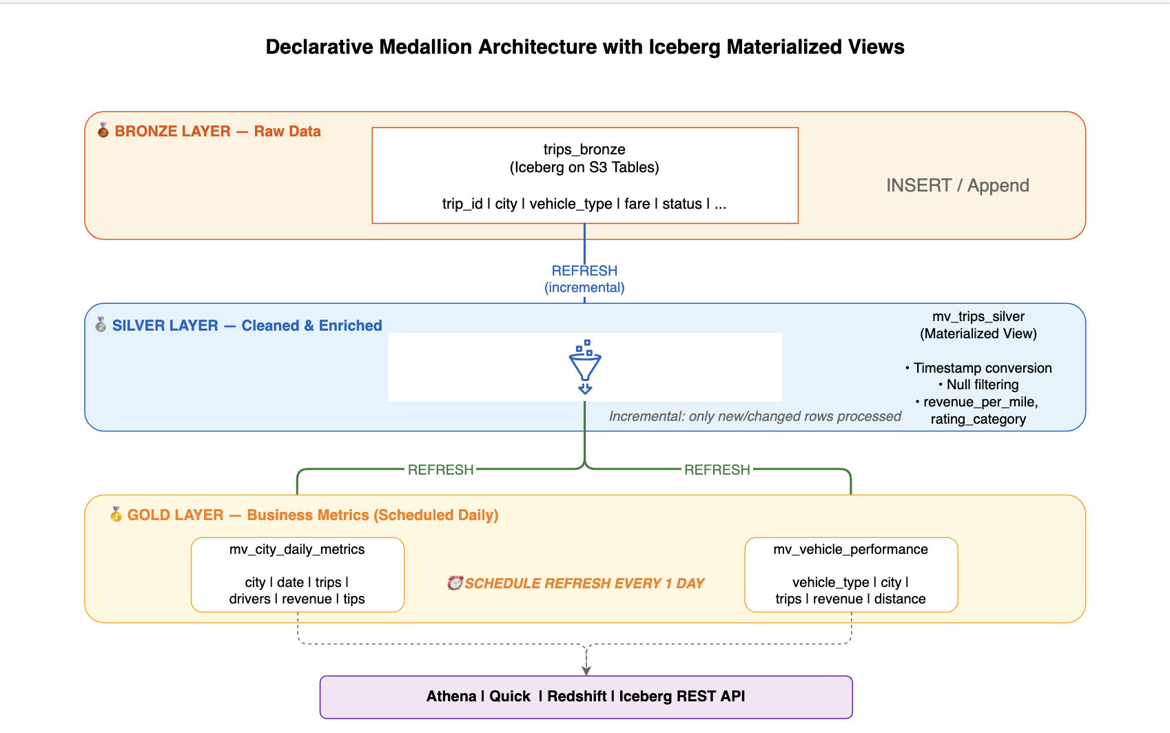
Figure 1: The three-tier medallion pipeline from the Bronze table through Silver and Gold materialized views to analytics consumers

Prerequisites

Before starting, verify that you have the following:

• An AWS account with permissions for Amazon SageMaker Unified Studio, AWS Glue, S3 Tables, and AWS Lake Formation.
• An Amazon SageMaker Unified Studio domain.

Step 1: Initialize the environment

Open the AWS Management Console and navigate to Amazon SageMaker.

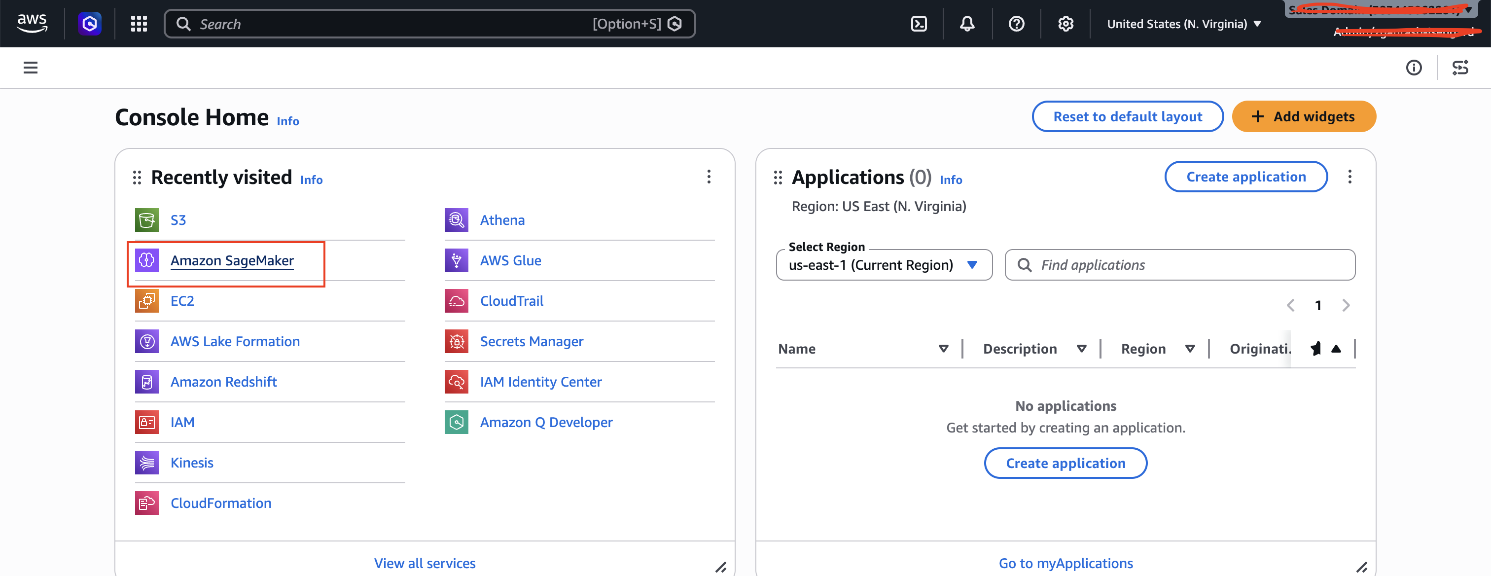
Figure 2: The Amazon SageMaker console landing page

Choose Get Started to set up Amazon SageMaker Unified Studio.

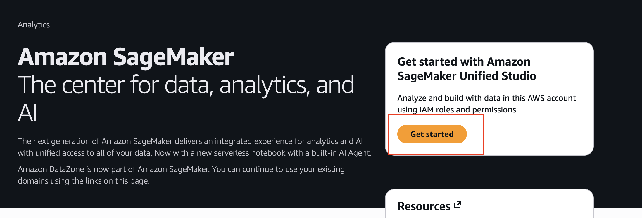
Figure 3: The Get Started page for setting up SageMaker Unified Studio

Choose Open to launch Amazon SageMaker Unified Studio.

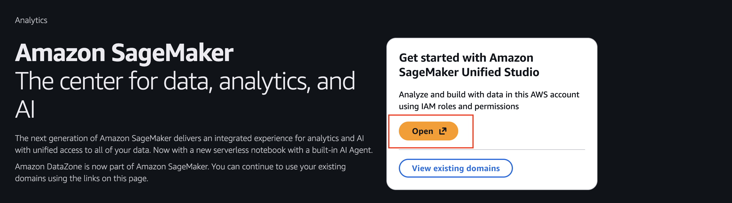
Figure 4: The option to open and launch SageMaker Unified Studio

After you’re in SageMaker Unified Studio, choose Data in the left pane to create the S3 Tables bucket (a managed Apache Iceberg feature of Amazon S3) and a database. Choose Add, then choose Create S3 Tables Catalog, and provide a catalog and a database name. Finally, choose Create Catalog.

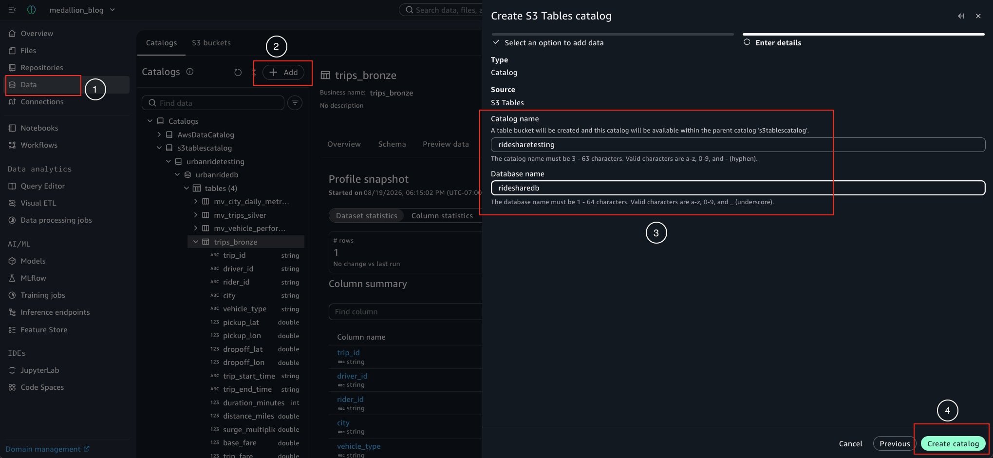
Figure 5: The Create S3 Tables Catalog dialog with catalog and database name fields

After the catalog creation is complete, in the left navigation pane, choose Notebooks.

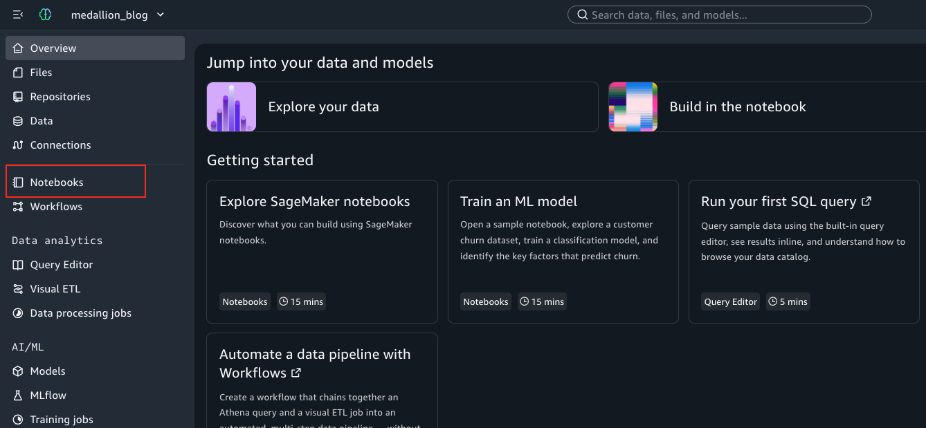
Figure 6: The Notebooks option in the SageMaker Unified Studio navigation pane

Choose Create Notebook.

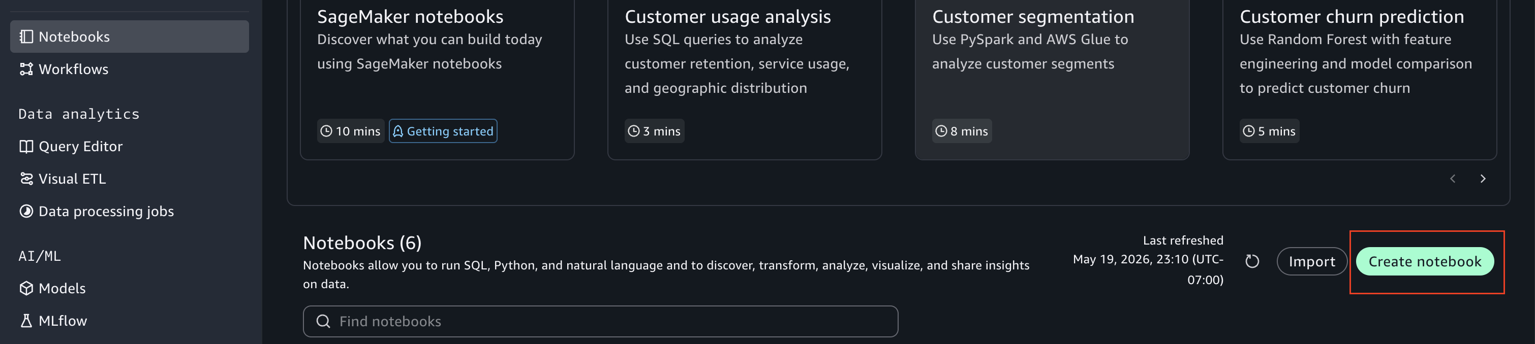
Figure 7: The Create Notebook button in SageMaker Unified Studio

Before using the notebook, select either Athena Spark or Glue Spark compute connection as the runtime engine for your notebook.

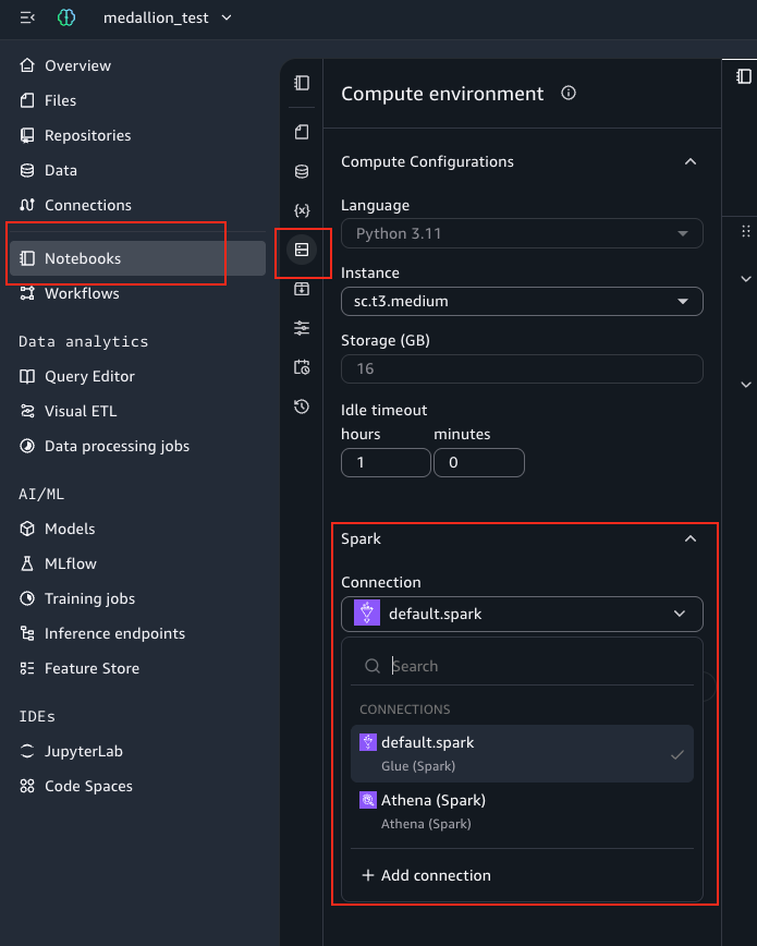
Figure 8: Selecting Athena Spark or Glue Spark as the notebook runtime engine

Use the following code samples in individual notebook cells. You can also provide transformation requirements in natural language, and the SageMaker Data Agent will generate SQL code for you.

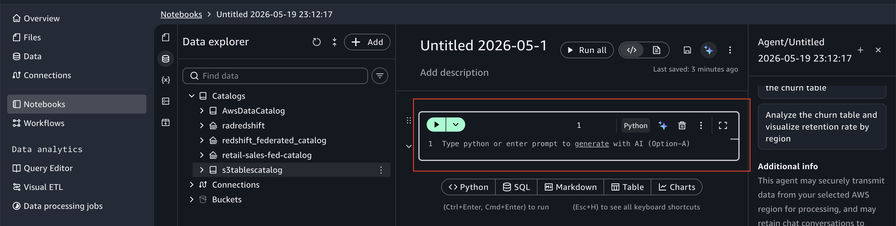
Figure 9: The SageMaker Data Agent generating SQL from a natural language request

Add each code block in a new cell by choosing the SQL button:

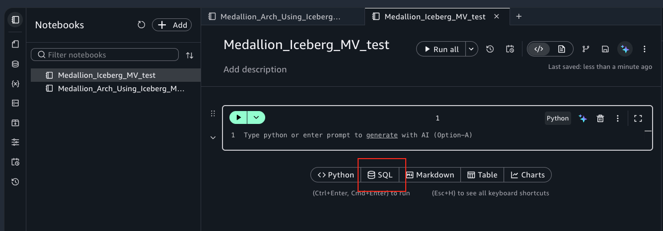
Figure 10: The SQL button for adding a code block to a notebook cell

Choose Athena Spark or Glue Spark as your compute from the cell menu.

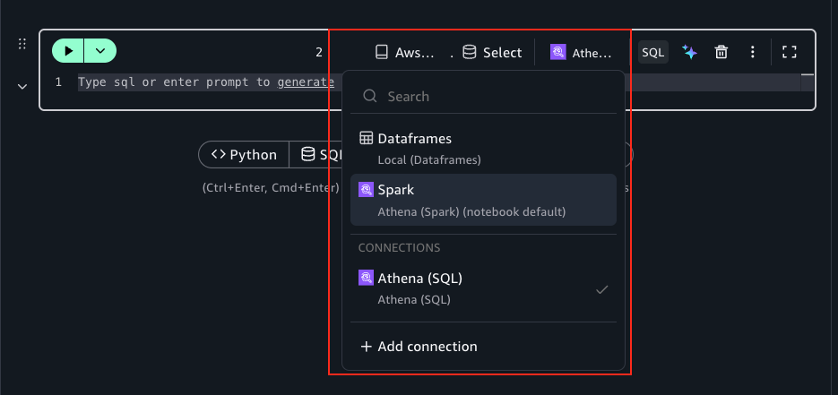
Figure 11: The compute selection in the notebook cell menu

If you encounter errors after cell execution, use the data agent chatbot or the Fix with AI button to resolve them.

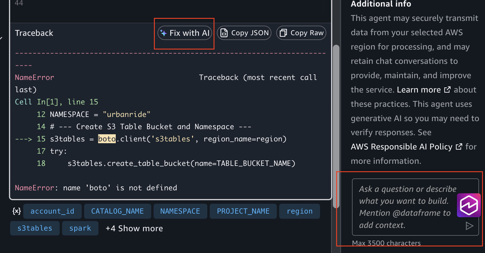
Figure 12: The Fix with AI button for resolving cell execution errors

Step 2: Ingest data into Bronze

Generate 300 realistic ride-sharing trips and insert them directly into the Bronze Iceberg table. This simulates a raw data ingestion layer. In production, you generally configure a streaming source or batch load based on your requirements.

Copy the following code into the first notebook cell (use a Python cell type).

import random
from datetime import datetime, timedelta

CITIES = {
    "San Francisco": {"lat_range": (37.70, 37.82), "lon_range": (-122.52, -122.38), "surge_prob": 0.3},
    "Austin": {"lat_range": (30.22, 30.40), "lon_range": (-97.80, -97.68), "surge_prob": 0.15},
    "Chicago": {"lat_range": (41.85, 41.95), "lon_range": (-87.70, -87.60), "surge_prob": 0.2},
    "Seattle": {"lat_range": (47.55, 47.68), "lon_range": (-122.40, -122.28), "surge_prob": 0.25},
}
VEHICLE_TYPES = ["UberX", "Comfort", "XL", "Black"]
PAYMENT_METHODS = ["credit_card", "debit_card", "apple_pay", "google_pay", "cash"]
STATUSES = ["completed"] * 4 + ["cancelled_rider", "cancelled_driver"]
BASE_FARES = {"UberX": 2.50, "Comfort": 3.50, "XL": 4.00, "Black": 7.00}
PER_MILE = {"UberX": 1.75, "Comfort": 2.25, "XL": 2.50, "Black": 3.75}
PER_MIN = {"UberX": 0.35, "Comfort": 0.45, "XL": 0.50, "Black": 0.65}

rows = []
for i in range(300):
    city_name = random.choice(list(CITIES.keys()))
    city = CITIES[city_name]
    vehicle = random.choice(VEHICLE_TYPES)
    duration = random.randint(5, 45)
    distance = round(random.uniform(1.0, 20.0), 1)
    surge = round(random.uniform(1.0, 2.5), 1) if random.random() < city["surge_prob"] else 1.0
    base = BASE_FARES[vehicle]
    fare = round((base + distance * PER_MILE[vehicle] + duration * PER_MIN[vehicle]) * surge, 2)
    tip = round(fare * random.choice([0, 0, 0.1, 0.15, 0.2, 0.25]), 2)
    status = random.choice(STATUSES)
    day = random.randint(0, 2)
    hour = random.choices(range(24),
        weights=[1,1,1,1,1,2,4,8,10,8,6,5,6,5,5,5,6,8,10,8,6,4,2,1])[0]
    trip_time = datetime(2025, 12, 1) + timedelta(days=day, hours=hour, minutes=random.randint(0, 59))

    rows.append((
        f"TRIP-{i+1:06d}",
        f"DRV-{random.randint(1000, 5000)}",
        f"RDR-{random.randint(10000, 99999)}",
        city_name, vehicle,
        round(random.uniform(*city["lat_range"]), 6),
        round(random.uniform(*city["lon_range"]), 6),
        round(random.uniform(*city["lat_range"]), 6),
        round(random.uniform(*city["lon_range"]), 6),
        trip_time.isoformat(),
        (trip_time + timedelta(minutes=duration)).isoformat(),
        duration, distance, surge, base, fare, tip, round(fare + tip, 2),
        random.choice(PAYMENT_METHODS),
        random.choice([None, 3, 4, 4, 5, 5, 5]) if status == "completed" else None,
        status,
    ))

schema = ("trip_id STRING, driver_id STRING, rider_id STRING, city STRING, "
    "vehicle_type STRING, pickup_lat DOUBLE, pickup_lon DOUBLE, "
    "dropoff_lat DOUBLE, dropoff_lon DOUBLE, trip_start_time STRING, "
    "trip_end_time STRING, duration_minutes INT, distance_miles DOUBLE, "
    "surge_multiplier DOUBLE, base_fare DOUBLE, trip_fare DOUBLE, "
    "tip_amount DOUBLE, total_amount DOUBLE, payment_method STRING, "
    "rating INT, status STRING")

df = spark.createDataFrame(rows, schema)
df.writeTo("{CATALOG_NAME}.{NAMESPACE_NAME}.trips_bronze").createOrReplace()

print(f"Created Table and Inserted {len(rows)} trips into Bronze layer")

Step 3: Explore Bronze

Run a preview on the bronze table. The output should look like the following screenshot:

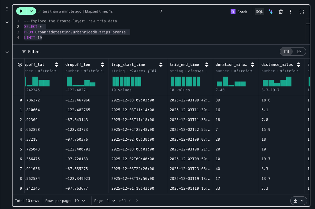
Figure 13: A preview of raw trip records in the Bronze table

You should see raw, unprocessed trip records with string timestamps and nullable fields. This is exactly what the Silver layer will clean up.

Now, verify the ingested data by querying the Bronze table for basic statistics.

SELECT COUNT(*) as total_trips, COUNT(DISTINCT city) as cities,
COUNT(DISTINCT vehicle_type) as vehicle_types,
MIN(trip_start_time) as earliest, MAX(trip_start_time) as latest
FROM ({CATALOG_NAME}.{NAMESPACE_NAME}.trips_bronze

The output should look like the following screenshot:

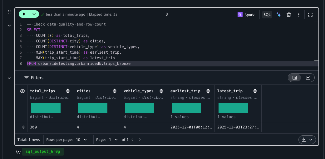
Figure 14: Bronze table statistics showing total trips, distinct cities, and vehicle types

Step 4: Create the Silver materialized view

This SQL statement defines the Silver layer as a materialized view that cleans, transforms, and derives new columns from the Bronze table. Note that this is only a definition. The system processes the data at refresh time.

CREATE MATERIALIZED VIEW IF NOT EXISTS {CATALOG_NAME}.{DATABASE}.mv_trips_silver
COMMENT 'Silver layer: Cleaned trip data with proper types and derived columns'
SCHEDULE REFRESH EVERY 1 DAY
AS
SELECT
trip_id, driver_id, rider_id, city, vehicle_type,
pickup_lat, pickup_lon, dropoff_lat, dropoff_lon,
CAST(trip_start_time AS TIMESTAMP) as trip_start_timestamp,
CAST(trip_end_time AS TIMESTAMP) as trip_end_timestamp,
duration_minutes, distance_miles, surge_multiplier,
base_fare, trip_fare, tip_amount, total_amount,
payment_method, rating, status,
CASE WHEN distance_miles > 0 THEN total_amount / distance_miles ELSE 0 END as revenue_per_mile,
CASE WHEN rating >= 4 THEN 'High' WHEN rating >= 3 THEN 'Medium' ELSE 'Low' END as rating_category
FROM {CATALOG_NAME}.{DATABASE}.trips_bronze
WHERE trip_id IS NOT NULL AND driver_id IS NOT NULL AND rider_id IS NOT NULL
AND total_amount >= 0 AND distance_miles >= 0

print("Silver MV created: urbanride.mv_trips_silver")

Verify the Silver layer output:

SELECT trip_id, city, vehicle_type, total_amount,
ROUND(revenue_per_mile, 2) as rev_per_mile, rating_category
FROM {CATALOG_NAME}.{DATABASE}.mv_trips_silver LIMIT 5

Notice how the Silver layer now has proper timestamps, derived revenue_per_mile, and rating categories: clean, typed, and ready for you to aggregate.

The output should look like the following screenshot:

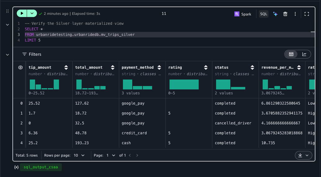
Figure 15: Silver materialized view results with typed timestamps and derived columns

Step 5: Create Gold materialized views

Gold materialized views read incrementally from the Silver materialized view. This is a nested materialized view pattern: a materialized view built on top of another materialized view.

Gold 1: City daily metrics

With this materialized view, you can aggregate trip data by city and date with a scheduled daily refresh.

CREATE MATERIALIZED VIEW IF NOT EXISTS {CATALOG_NAME}.urbanride.mv_city_daily_metrics
COMMENT 'Gold layer: Daily aggregated metrics by city'
SCHEDULE REFRESH EVERY 1 DAY
AS
SELECT
city, DATE(trip_start_timestamp) as trip_date,
COUNT(*) as total_trips,
COUNT(DISTINCT driver_id) as active_drivers,
COUNT(DISTINCT rider_id) as active_riders,
SUM(total_amount) as total_revenue,
SUM(distance_miles) as total_distance,
SUM(tip_amount) as total_tips
FROM {CATALOG_NAME}.{DATABASE}.mv_trips_silver
WHERE status="completed"
GROUP BY city, DATE(trip_start_timestamp)

print("Gold MV created: mv_city_daily_metrics (reads from Silver MV, refreshes daily)")

Gold 2: Vehicle performance

With this materialized view, you can aggregate performance metrics by vehicle type and city.

CREATE MATERIALIZED VIEW IF NOT EXISTS {CATALOG_NAME}.{DATABASE}.mv_vehicle_performance
COMMENT 'Gold layer: Vehicle type performance metrics'
SCHEDULE REFRESH EVERY 1 DAY
AS
SELECT
vehicle_type, city,
COUNT(*) as trip_count,
SUM(total_amount) as total_revenue,
SUM(distance_miles) as total_distance,
SUM(tip_amount) as total_tips
FROM {CATALOG_NAME}.{DATABASE}.mv_trips_silver
WHERE status="completed"
GROUP BY vehicle_type, city

print("Gold MV created: mv_vehicle_performance (reads from Silver MV, refreshes daily)")

Dependency chain

The complete pipeline dependency is:

trips_bronze (table)
└── mv_trips_silver (materialized view)
    ├── mv_city_daily_metrics (MV on MV, daily schedule)
    └── mv_vehicle_performance (MV on MV, daily schedule)

Each layer is defined by a single SQL statement. There are no DAGs to maintain, no job definitions to deploy, and no watermark tracking to implement.

Step 6: Query the Gold layer

Query the Gold materialized views to see aggregated business metrics.

City daily metrics Gold table

SELECT city, trip_date, total_trips, active_drivers,
ROUND(total_revenue, 2) as revenue,
ROUND(total_revenue / total_trips, 2) as avg_per_trip
FROM {CATALOG_NAME}.{DATABASE}.mv_city_daily_metrics
ORDER BY trip_date DESC, revenue DESC LIMIT 15

The output should look like the following screenshot:

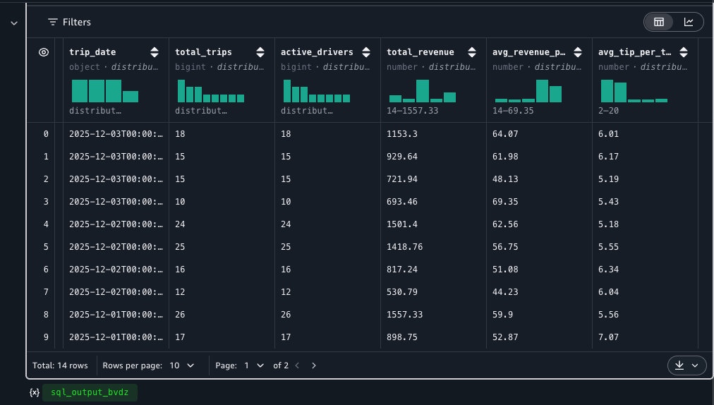
Figure 16: City daily metrics from the Gold materialized view

Vehicle performance Gold table

SELECT vehicle_type, city, trip_count,
ROUND(total_revenue, 2) as revenue,
ROUND(total_revenue / trip_count, 2) as avg_per_trip
FROM {CATALOG_NAME}.{DATABASE}.mv_vehicle_performance
ORDER BY revenue DESC

The output should look like the following screenshot:

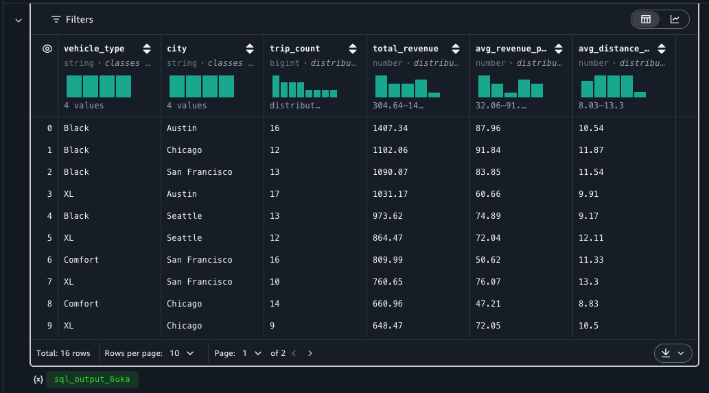
Figure 17: Vehicle performance metrics from the Gold materialized view

The Gold layer gives you pre-aggregated, business-ready metrics without writing aggregation jobs.

Step 7: Data propagation demo

This section demonstrates how changes propagate through the layers using INSERT, UPDATE (MERGE), and DELETE operations followed by incremental refresh. In production, the scheduled refresh handles this automatically. We trigger it manually here for demonstration purposes.

INSERT new records

Insert new trip records into the Bronze table.

INSERT INTO {CATALOG_NAME}.{DATABASE}.trips_bronze VALUES
('DEMO_TRIP_001', 'DRIVER_999', 'RIDER_888', 'Seattle', 'UberX',
47.6062, -122.3321, 47.6205, -122.3493,
'2024-12-15 14:30:00', '2024-12-15 14:50:00',
20, 5.2, 1.0, 10.0, 15.0, 3.0, 18.0, 'credit_card', 5, 'completed'),
('DEMO_TRIP_002', 'DRIVER_888', 'RIDER_777', 'Seattle', 'XL',
47.6101, -122.3300, 47.6550, -122.3080,
'2024-12-15 15:00:00', '2024-12-15 15:35:00',
35, 8.5, 1.5, 15.0, 30.0, 5.0, 35.0, 'cash', 4, 'completed'),
('DEMO_TRIP_003', 'DRIVER_777', 'RIDER_666', Portland, 'Comfort',
30.2672, -97.7431, 30.2800, -97.7400,
'2024-12-15 16:00:00', '2024-12-15 16:15:00',
15, 3.0, 1.0, 8.0, 12.0, 2.0, 14.0, 'credit_card', 5, 'completed')

print("Inserted 3 new trips into Bronze")

Refresh Silver (incremental)

Refresh the Silver materialized view. Iceberg materialized view processes only three new records.

REFRESH MATERIALIZED VIEW {CATALOG_NAME}.{DATABASE}.mv_trips_silver"

Verify the new records propagated

SELECT trip_id, city, total_amount, ROUND(revenue_per_mile, 2) as rev_per_mile, rating_category
FROM {CATALOG_NAME}.{DATABASE}.mv_trips_silver
WHERE trip_id LIKE 'DEMO_TRIP_%' ORDER BY trip_id

The output should look like the following screenshot:

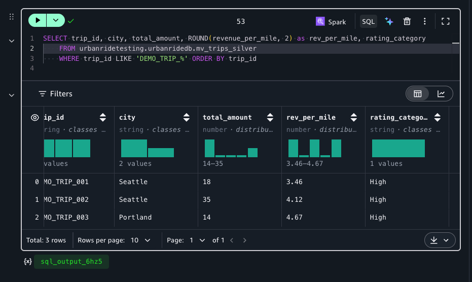
Figure 18: The Silver materialized view showing the three newly inserted demo trips

Refresh Gold (cascading from the Silver materialized view)

Refresh the Gold materialized view. It reads from the refreshed Silver materialized view and processes only the incremental changes.

REFRESH MATERIALIZED VIEW {CATALOG_NAME}.{DATABASE}.mv_city_daily_metrics

Verify the Gold layer reflects the new trips

SELECT city, trip_date, total_trips, ROUND(total_revenue, 2) as revenue
FROM {CATALOG_NAME}.{DATABASE}.mv_city_daily_metrics
WHERE trip_date="2024-12-15" ORDER BY city

The output should look like the following screenshot:

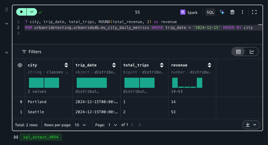
Figure 19: City daily metrics reflecting the new trips for 2024-12-15

UPDATE through MERGE

Use MERGE to update existing records in Bronze, then refresh incrementally.

MERGE INTO {CATALOG_NAME}.{DATABASE}.trips_bronze AS target
USING (SELECT 'DEMO_TRIP_002' as trip_id, 5 as new_rating, 20.0 as new_tip) AS source
ON target.trip_id = source.trip_id
WHEN MATCHED THEN UPDATE SET
target.rating = source.new_rating,
target.tip_amount = source.new_tip,
target.total_amount = target.trip_fare + source.new_tip

Refresh Silver and verify

REFRESH MATERIALIZED VIEW {CATALOG_NAME}.{DATABASE}.mv_trips_silver")

SELECT trip_id, rating, rating_category, tip_amount, total_amount,
ROUND(revenue_per_mile, 2) as rev_per_mile
FROM {CATALOG_NAME}.{DATABASE}.mv_trips_silver WHERE trip_id = 'DEMO_TRIP_002'

print("UPDATE propagated: rating 4->5, tip $5->$20, total $35->$50")

The output should look like the following screenshot:

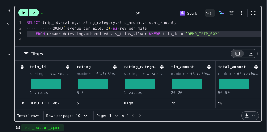
Figure 20: The Silver materialized view showing the updated rating and tip for the demo trip

Step 8: Cleanup

Drop materialized views, tables, the namespace, and delete the S3 Tables bucket to fully clean up resources.

# Drop MVs (Gold first, then Silver, due to dependency order)
spark.sql(f"DROP MATERIALIZED VIEW IF EXISTS {CATALOG_NAME}.{DATABASE}.mv_city_daily_metrics")
spark.sql(f"DROP MATERIALIZED VIEW IF EXISTS {CATALOG_NAME}.{DATABASE}.mv_vehicle_performance")
spark.sql(f"DROP MATERIALIZED VIEW IF EXISTS {CATALOG_NAME}.{DATABASE}.mv_trips_silver")
print("All materialized views dropped")

# Drop base table
spark.sql(f"DROP TABLE IF EXISTS {CATALOG_NAME}.{DATABASE}.trips_bronze")
print("Base table dropped")

# Drop the namespace
spark.sql(f"DROP NAMESPACE IF EXISTS {CATALOG_NAME}.{DATABASE} ")
print("Namespace dropped")

# Delete the S3 table bucket
import boto3
s3tables_client = boto3.client("s3tables")

# List and delete all remaining tables in the bucket
tables_response = s3tables_client.list_tables(
    tableBucketARN=TABLE_BUCKET_ARN, namespace="{DATABASE}"
)
for table in tables_response.get("tables", []):
    s3tables_client.delete_table(
        tableBucketARN=TABLE_BUCKET_ARN, namespace="{DATABASE}", name=table['name']
    )
    print(f" Deleted table: {table['name']}")

# Delete the namespace and bucket
s3tables_client.delete_namespace(tableBucketARN=TABLE_BUCKET_ARN, namespace="urbanride")
s3tables_client.delete_table_bucket(tableBucketARN=TABLE_BUCKET_ARN)
print(f"S3 table bucket deleted: {TABLE_BUCKET_NAME}")

Limitations and considerations

While materialized views remove most orchestration code, note the following:

1. No sub-hour freshness. The minimum schedule granularity is one hour (SCHEDULE REFRESH EVERY 1 HOUR).
2. Cascading refresh isn’t automatic. Refreshing Silver doesn’t trigger Gold in the same operation. Each layer refreshes on its own schedule or must be triggered sequentially.
3. Deletes require a FULL refresh. An incremental REFRESH that feeds the Silver layer detects inserts and updates through Iceberg metadata but cannot detect row removals. Use REFRESH ... FULL when delete propagation is needed.
4. SQL subset only. Some window functions, user-defined functions (UDFs), and complex expressions might not be supported in materialized view definitions.
5. Schema evolution requires recreation. If the source schema changes in a way that affects the materialized view definition, you must drop and recreate it.
6. AWS-specific extension. Iceberg materialized views are not part of the open-source Apache Iceberg specification. They aren’t portable to non-AWS environments.

Pricing

AWS bills materialized view auto-refresh at USD $0.44 per DPU-hour (4 vCPU, 16 GB memory), billed per second with a 1-minute minimum. When you configure scheduled refresh, the AWS Glue Data Catalog uses managed Spark compute to incrementally update the materialized view. You pay only for the compute time of each refresh run.

There are no separate charges for storing materialized view metadata in the Data Catalog (covered under standard catalog pricing: first million objects at no additional cost, then $1.00 per 100K objects/month). The materialized view data itself is stored as Iceberg files in S3 Tables or Amazon S3, charged at standard Amazon S3 storage rates.

Manual refreshes triggered from Spark (through Amazon Athena, Amazon EMR, or AWS Glue notebooks) are billed under those services’ respective compute pricing rather than the materialized view auto-refresh rate. For the latest pricing details, see the AWS Glue pricing page.

Estimated cost for this tutorial: Running through all steps once with 300 records typically consumes less than 0.5 DPU-hours total (~$0.22 in AWS Glue compute plus negligible Amazon S3 storage).

Summary

In this post, you built a Bronze → Silver → Gold medallion architecture using three SQL statements with nested materialized views and no orchestration code. The full pipeline creation took under 2 minutes, and incremental refreshes processed only changed data with no watermarks, no DAGs, no CDC plumbing.

To get started with your own data, create an Amazon SageMaker Unified Studio project, define your Bronze table, and express your transformation logic as Iceberg materialized views. For more information, see the Apache Iceberg materialized views documentation in the AWS Glue Developer Guide.

References

Using materialized views with AWS Glue

Query AWS Glue Data Catalog materialized views

Using materialized views with Amazon EMR

Working with Amazon S3 Tables and table buckets

About the authors