Build declarative ETL pipelines with AWS Glue 6.0

Data teams commonly build the extract, transform, and load (ETL) pipelines that turn raw order events into analyst-ready aggregates as a bronze, silver, and gold sequence, the medallion architecture. Bronze holds raw ingested records, silver holds cleaned and validated data, and gold holds the business-level aggregates that analysts query. Today you build this on AWS Glue with an orchestrator such as Amazon Managed Workflows for Apache Airflow (Amazon MWAA) or AWS Step Functions coordinating the stages. Many teams run production pipelines exactly this way. As a pipeline grows, the coordination work grows with it: you wire job dependencies, manage intermediate checkpoints, and add retry logic stage by stage.

AWS Glue 6.0, powered by Apache Spark 4.1, introduces Spark Declarative Pipelines (SDP), which simplifies this further. Instead of orchestrating jobs by hand, you declare what each dataset should contain and let the declarative framework resolve dependencies, manage checkpoints, and orchestrate execution order automatically. The result runs as a single declarative job, with no manual directed acyclic graph (DAG) wiring or imperative orchestration code.

In this post, you build a single AWS Glue 6.0 job that turns raw order records into validated, aggregated, analytics-ready tables through the bronze, silver, and gold sequence. You do this without writing any orchestration logic. This walkthrough uses the AWS Command Line Interface (AWS CLI), and the same operations are available through the AWS SDKs.

Solution overview

You build a single AWS Glue 6.0 job that reads raw order records from a CSV file in Amazon Simple Storage Service (Amazon S3). The job flows them through three declared datasets. These are a bronze materialized view (ingest as-is), a silver materialized view (type, validate, and classify), and a gold SQL materialized view (aggregate by region). With AWS Glue Data Catalog integration turned on, all three land as Data Catalog tables, queryable with standard SQL tooling such as Amazon Athena. SDP resolves the dependency order from the dataset references in your code, so you never orchestrate the steps yourself.

Before and after: Imperative compared to declarative

Before you build the pipeline, let’s understand this new way of writing ETL pipelines with a quick comparison of the imperative and declarative approaches.

With the imperative approach, you need three AWS Glue jobs, plus an orchestrator to handle sequencing and error handling. A typical pipeline therefore has two layers: an orchestration layer and the ETL processing layer. The following diagram shows this two-layer imperative pipeline.

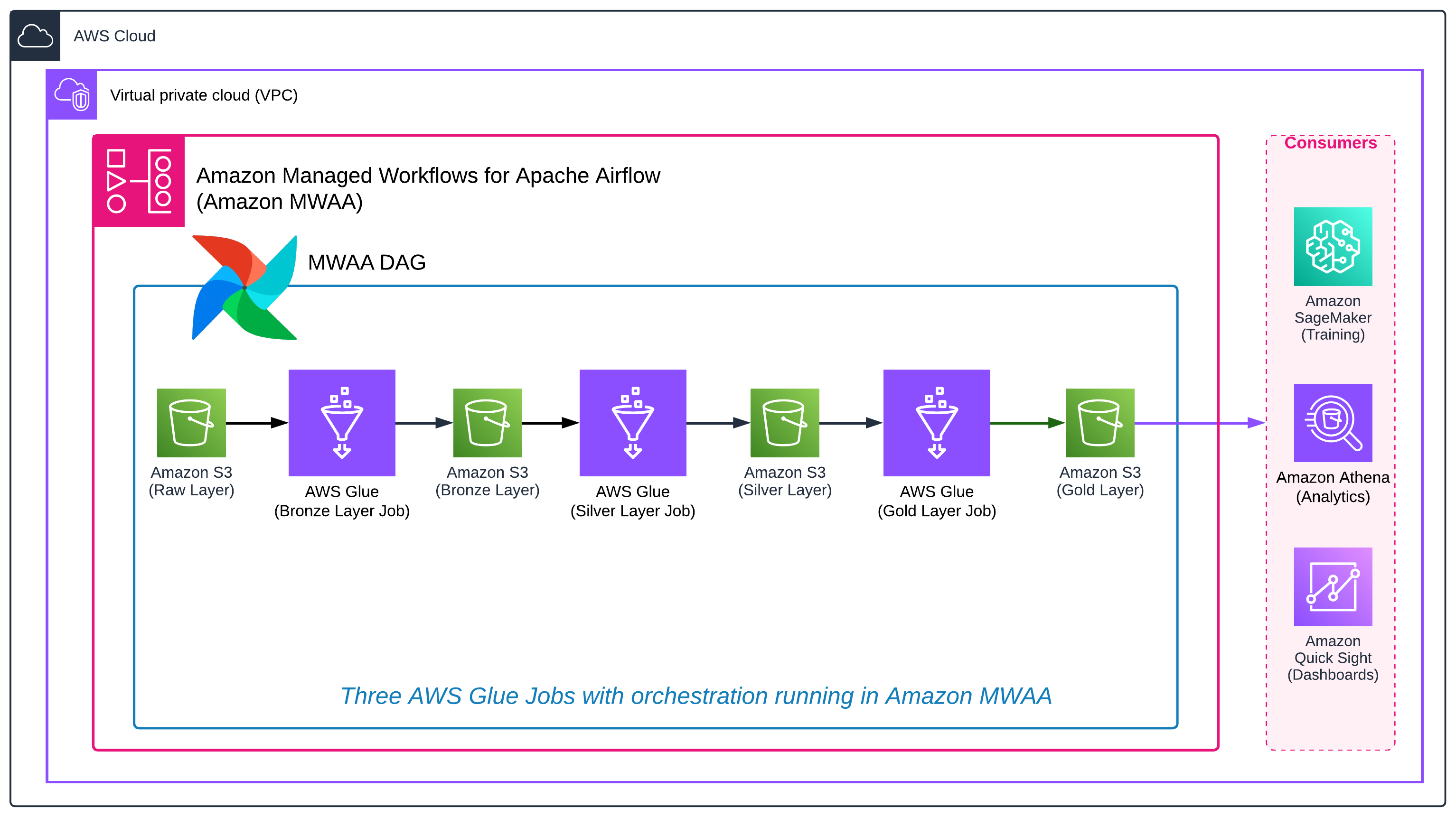
Figure 1: The two-layer imperative pipeline, with three AWS Glue jobs coordinated by an orchestrator.

Compared to that, the declarative approach runs as a single ETL job with SDP. The following diagram mirrors the previous one, but here it’s a single AWS Glue ETL job instead of three jobs plus an orchestrator.

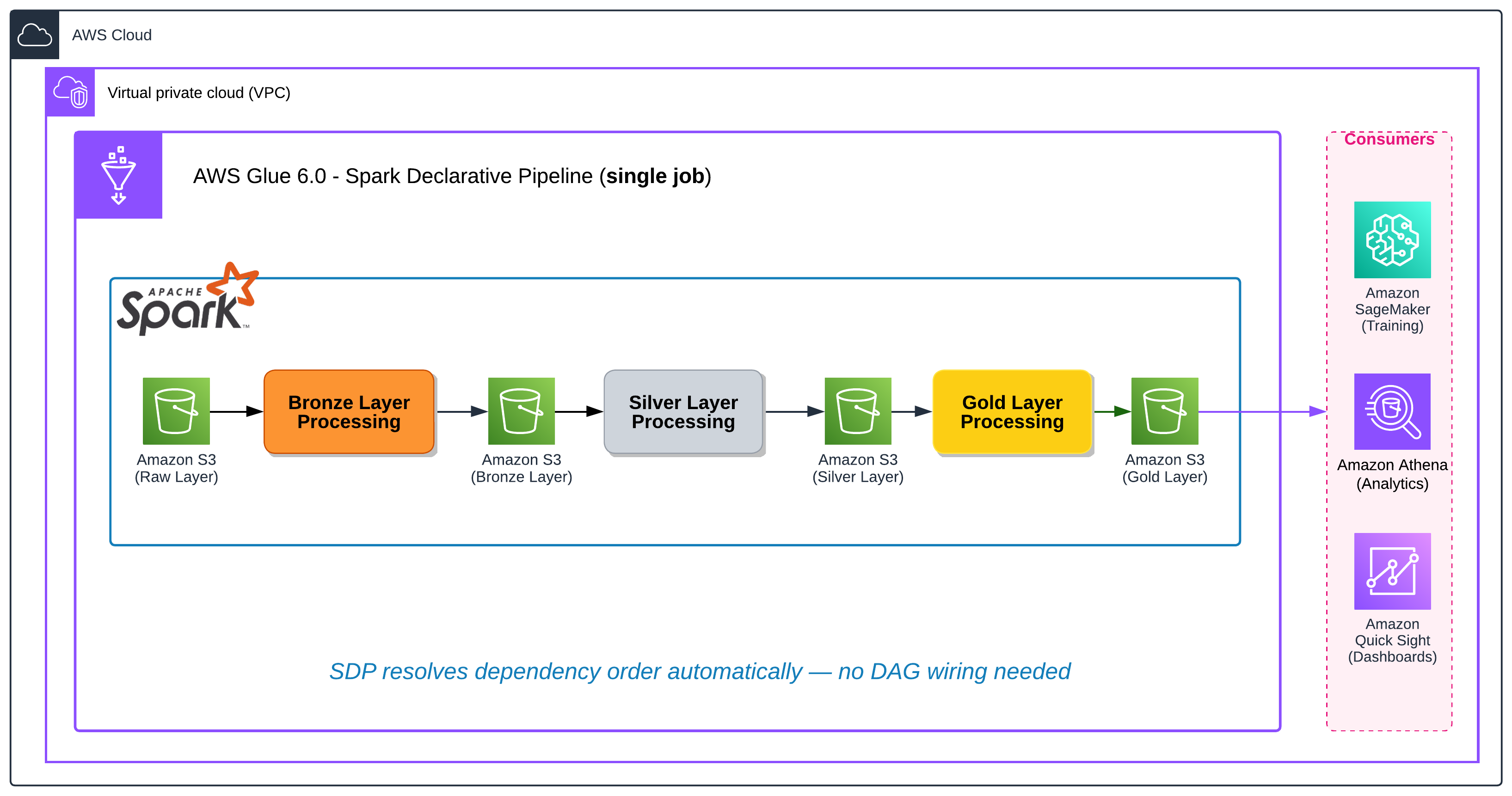
Figure 2: The declarative pipeline, a single AWS Glue job running the bronze, silver, and gold layers with SDP.

The declarative approach reduces more than the number of jobs. It removes the boilerplate that surrounds them. You no longer hand-wire a DAG, manage per-stage checkpoint paths, or add retry logic stage by stage. SDP derives the dependency graph from your table references and manages execution for you. You can still invoke an SDP job from an orchestrator when a broader workflow calls for it, but the pipeline’s internal coordination is no longer code you write and maintain.

SDP separates the what from the how: you declare datasets (the outputs you want), and SDP builds the flows that produce them and runs them as one pipeline, resolving dependencies and execution order automatically.

You declare these abstractions through Python decorators. This post covers three of them, @dp.table, @dp.materialized_view, and @dp.temporary_view, each with its own purpose:

• @dp.table defines a streaming table, which processes new data incrementally on each run. Typical use cases are raw event ingestion and change data capture (CDC) feeds.
• @dp.materialized_view defines a materialized view for batch use cases. Today, this dataset type fully recomputes on each run. Common uses include parsing, aggregations, and machine learning (ML) feature engineering.
• @dp.temporary_view is for temporary computations and aggregations. It’s pipeline-scoped and isn’t persisted outside the pipeline. Use it for enrichment lookups and subqueries.

Streaming tables append only new arrivals. Materialized views fully recompute. This post uses @dp.materialized_view for all three layers to keep the walkthrough focused. In production, you would typically use @dp.table for the bronze layer to process only new files as they arrive rather than re-reading the full source each run.

The following table compares the two approaches and how the declarative approach addresses each concern:

Table 1: Imperative compared to declarative approaches for a three-layer ETL pipeline.

Running and refreshing the pipeline

When you rerun a pipeline, you don’t always want the same work to happen. Sometimes you only want to confirm the pipeline is well-formed before spending compute. Other times you want to run it but recompute only the datasets that changed rather than the entire graph. SDP handles both cases through two independent controls, and it helps to keep them separate:

• Execution mode (the spark.glue.sdp.jobMode key) answers run or only validate?
• Refresh scope (the spark.glue.sdp.runMode key) answers given that I’m running, what do I recompute?

Execution mode. VALIDATE runs the pipeline in dry-run mode: SDP checks the YAML syntax, dependency resolution, and SQL and Python compilation without writing any data. Use it to verify your pipeline is well-formed before committing compute. RUN (the default) executes the pipeline normally, resolving the dependency graph and materializing datasets.

# Dry run: validate the graph, write nothing
aws glue start-job-run \
  --job-name "${JOB_NAME}" \
  --arguments '{"--conf":"spark.glue.sdp.jobMode=VALIDATE"}' \
  --region "${AWS_REGION}"

# Normal execution
aws glue start-job-run \
  --job-name "${JOB_NAME}" \
  --arguments '{"--conf":"spark.glue.sdp.jobMode=RUN"}' \
  --region "${AWS_REGION}"

Refresh scope. By default, a RUN recomputes every materialized view. You can narrow or widen that with spark.glue.sdp.runMode:

• --refresh <datasets> updates only the named datasets (comma-separated, no spaces).
• --full-refresh <datasets> resets and recomputes only the named datasets (for streaming tables, this also clears their checkpoints).
• --full-refresh-all resets and recomputes every dataset in the pipeline.

# Selective refresh of named datasets
aws glue start-job-run \
  --job-name "${JOB_NAME}" \
  --arguments '{"--conf":"spark.glue.sdp.jobMode=RUN --conf spark.glue.sdp.runMode=--refresh silver_orders,gold_sales_summary"}' \
  --region "${AWS_REGION}"

# Full reset and recompute of the entire pipeline
aws glue start-job-run \
  --job-name "${JOB_NAME}" \
  --arguments '{"--conf":"spark.glue.sdp.jobMode=RUN --conf spark.glue.sdp.runMode=--full-refresh-all"}' \
  --region "${AWS_REGION}"

Selective refresh is useful during development, so you can iterate on a single layer without reprocessing the entire graph. Note that --refresh and --full-refresh each take an explicit list of datasets. To reset the whole pipeline, use --full-refresh-all. Because materialized views hold no incremental state, resetting a materialized view and refreshing it both fully recompute it. The reset-versus-refresh distinction matters for streaming tables, where a refresh processes only new data and a reset clears the checkpoint and reprocesses from scratch.

The multiple values are passed as a single --conf argument string ("spark.glue.sdp.jobMode=RUN --conf spark.glue.sdp.runMode=..."). This is the serialization the AWS Glue SDP mode expects for the run.

Materialized views: Batch transforms with automatic dependency resolution

Materialized views recompute their full result set on each run. SDP infers dependencies from table references: in this pipeline, silver_orders references bronze_orders, so SDP runs bronze first, as shown in the following diagram.

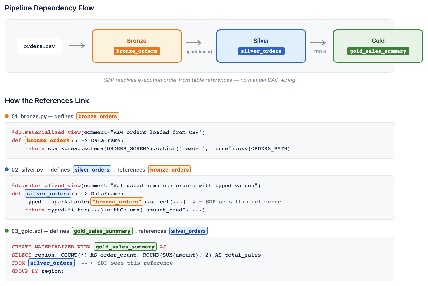
Figure 3: SDP infers the dependency order from table references and runs bronze before silver.

The core pattern is a decorated function that returns a DataFrame:

@dp.materialized_view(comment="Raw orders loaded from CSV")
def bronze_orders() -> DataFrame:
    return spark.read.schema(ORDERS_SCHEMA).option("header", "true").csv(ORDERS_PATH)

The silver layer references bronze_orders through spark.table("bronze_orders"), with no explicit dependency declaration. SDP builds the DAG by analyzing table references in your code and runs bronze first automatically.

Bronze reads every column as a string by design: the bronze layer preserves raw source data without coercion. Type casting, validation, and filtering happen in the silver layer.

SQL and Python coexistence

SDP supports both Python and SQL definitions in the same pipeline project. A SQL materialized view can reference a Python-defined table directly, for example the gold layer aggregating the silver table:

CREATE MATERIALIZED VIEW gold_sales_summary
COMMENT 'Completed-order metrics by region'
AS
SELECT
  region,
  COUNT(*) AS order_count,
  CAST(ROUND(SUM(amount), 2) AS DECIMAL(10, 2)) AS total_sales,
  CAST(ROUND(AVG(amount), 2) AS DECIMAL(10, 2)) AS average_order_value
FROM silver_orders
GROUP BY region;

In this post, Python files define ingestion and validation logic, and SQL files define reporting views and aggregations. SDP discovers both through the libraries glob pattern in the pipeline specification and resolves the cross-language dependencies automatically. The complete source for all three layers follows in the step-by-step walkthrough.

Build the pipeline: Step by step

The rest of this post is a hands-on walkthrough. You build a single AWS Glue 6.0 job that reads orders.csv and processes it through the bronze, silver, and gold layers. The steps are:

1. Prerequisites: AWS account, AWS Identity and Access Management (IAM) role, and S3 bucket.
2. Set up sample data: create orders.csv and upload it to Amazon S3.
3. Build the pipeline files (the spark-pipeline.yml specification plus the three transformation files).
4. Package the pipeline into a zip and upload it to Amazon S3.
5. Create the database: a Data Catalog database with an S3 location.
6. Configure the job: create the AWS Glue 6.0 job with the SDP flag.
7. Validate: run in dry-run mode to verify the graph.
8. Run the pipeline to materialize all datasets.
9. Query results: inspect the tables with Amazon Athena.
10. Clean up: delete the resources you created.

Step 1 – Prerequisites

To follow along, you need:

• An AWS account with access to AWS Glue 6.0.
• A dedicated IAM role trusted by glue.amazonaws.com (set up in the following section).
• A private, encrypted Amazon S3 bucket with Block Public Access enabled.
• The AWS CLI configured with credentials for a non-production account.

IAM role for the pipeline

Create a role that AWS Glue can assume, with the following trust policy:

{
  "Version": "2012-10-17",
  "Statement": [{
    "Effect": "Allow",
    "Principal": { "Service": "glue.amazonaws.com" },
    "Action": "sts:AssumeRole"
  }]
}

Attach the AWS managed policy AWSGlueServiceRole, which grants the AWS Glue Data Catalog and Amazon CloudWatch Logs access the job needs. Then add an inline policy that scopes Amazon S3 access to your bucket, covering the input data, the pipeline zip, the pipeline storage (state) path, and the warehouse location:

{
  "Version": "2012-10-17",
  "Statement": [{
    "Effect": "Allow",
    "Action": ["s3:GetObject", "s3:PutObject", "s3:DeleteObject", "s3:ListBucket"],
    "Resource": [
      "arn:aws:s3:::amzn-s3-demo-bucket",
      "arn:aws:s3:::amzn-s3-demo-bucket/*"
    ]
  }]
}

For a full breakdown of the baseline permissions, see Setting up IAM permissions for AWS Glue.

Set the walkthrough variables

Set the following variables, replacing the example values (us-east-1, amzn-s3-demo-bucket, the account ID 111122223333, and the role name) with your own:

export AWS_REGION="us-east-1"
export BUCKET="amzn-s3-demo-bucket"
export PREFIX="simple-sdp-demo"
export DATABASE="simple_sdp_demo_db"
export ROLE_ARN="arn:aws:iam::111122223333:role/AWSGlueServiceRole-sdp-demo"
export JOB_NAME="simple-sdp-demo"

Step 2 – Set up sample data

The pipeline reads a CSV of order records. Save the following as orders.csv:

order_id,customer_id,region,amount,status,order_ts
O-1001,C-101,EMEA,120.50,COMPLETE,2026-07-23T08:00:00Z
O-1002,C-102,AMER,750.00,COMPLETE,2026-07-23T08:15:00Z
O-1003,C-103,EMEA,-10.00,INVALID,2026-07-23T08:30:00Z
O-1004,C-104,APAC,320.25,COMPLETE,2026-07-23T09:00:00Z
O-1005,C-105,AMER,250.00,COMPLETE,2026-07-23T09:15:00Z
O-1006,C-106,EMEA,90.00,COMPLETE,2026-07-23T09:30:00Z

Upload the file to the input/ location under your project prefix, which is where the bronze layer reads it (the ORDERS_PATH in 01_bronze.py, shown in Step 3). Use the variables you exported in Step 1:

aws s3 cp orders.csv \
  "s3://${BUCKET}/${PREFIX}/input/orders.csv" \
  --region "${AWS_REGION}"

The file includes one invalid order (O-1003, a negative amount), which the silver layer filters out to demonstrate the validation step. The AMER and EMEA regions each have two completed orders, so the gold layer’s order_count and average_order_value are meaningful aggregations rather than single-row passthroughs.

Step 3 – Build the pipeline files

The pipeline project uses the structure introduced earlier: a transformations/ folder holding the three layer definitions (01_bronze.py, 02_silver.py, 03_gold.sql), plus the spark-pipeline.yml specification. The following screenshot shows this layout in a code editor.

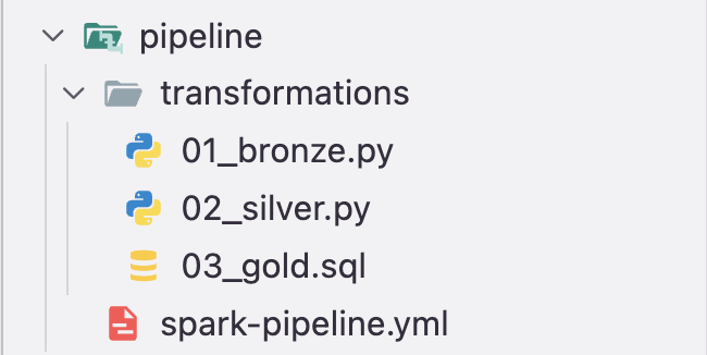
Figure 4: The pipeline project layout in a code editor.

The complete contents of each file follow.

3a. spark-pipeline.yml

The specification names the pipeline, points to the Data Catalog database, configures state storage, and discovers transformation files. As with the transformation files, it uses the __DATABASE__, __BUCKET__, and __PREFIX__ tokens, which you substitute at packaging time in Step 4:

name: simple_sdp_demo
catalog: spark_catalog
database: __DATABASE__
storage: s3://__BUCKET__/__PREFIX__/state/
libraries:
  - glob:
      include: transformations/**
configuration:
  spark.sql.shuffle.partitions: "4"

3b. transformations/01_bronze.py

Bronze preserves the raw source as strings. No coercion, no filtering:

"""Bronze layer: preserve source order records as strings."""
from pyspark import pipelines as dp
from pyspark.sql import DataFrame, SparkSession
from pyspark.sql.types import StringType, StructField, StructType

spark = SparkSession.active()

ORDERS_PATH = "s3://__BUCKET__/__PREFIX__/input/orders.csv"

ORDERS_SCHEMA = StructType([
    StructField("order_id", StringType(), True),
    StructField("customer_id", StringType(), True),
    StructField("region", StringType(), True),
    StructField("amount", StringType(), True),
    StructField("status", StringType(), True),
    StructField("order_ts", StringType(), True),
])


@dp.materialized_view(comment="Raw orders loaded from CSV")
def bronze_orders() -> DataFrame:
    return (
        spark.read
        .schema(ORDERS_SCHEMA)
        .option("header", "true")
        .csv(ORDERS_PATH)
    )

The path uses the tokens __BUCKET__ and __PREFIX__ rather than hardcoded values. AWS Glue reads these files from the packaged zip at runtime, so shell variables like ${BUCKET} are not expanded inside them. You substitute the tokens with your real values when you package the project in Step 4, which keeps every file consistent with the variables you exported in Step 1.

3c. transformations/02_silver.py

Silver casts types, filters to complete orders with positive amounts, and derives an amount_band classification:

"""Silver layer: type, validate, and classify complete orders."""
from pyspark import pipelines as dp
from pyspark.sql import DataFrame, SparkSession
from pyspark.sql.functions import col, to_timestamp, trim, when

spark = SparkSession.active()


@dp.materialized_view(comment="Validated complete orders with typed values")
def silver_orders() -> DataFrame:
    typed = (
        spark.table("bronze_orders")
        .select(
            trim(col("order_id")).alias("order_id"),
            trim(col("customer_id")).alias("customer_id"),
            trim(col("region")).alias("region"),
            col("amount").cast("double").alias("amount"),
            trim(col("status")).alias("status"),
            to_timestamp("order_ts", "yyyy-MM-dd'T'HH:mm:ss'Z'").alias("order_ts"),
        )
        .filter(
            col("order_id").isNotNull()
            & col("region").isNotNull()
            & col("order_ts").isNotNull()
            & (col("status") == "COMPLETE")
            & (col("amount") > 0)
        )
    )
    return typed.select(
        "*",
        when(col("amount") >= 500, "large")
        .when(col("amount") >= 100, "medium")
        .otherwise("small")
        .alias("amount_band"),
    )

Silver reads bronze with spark.table("bronze_orders"), so SDP infers the dependency and runs bronze first. Two details matter here:

• The to_timestamp call passes an explicit format, "yyyy-MM-dd'T'HH:mm:ss'Z'". The source timestamps are ISO 8601 with a Z suffix. Giving the format treats Z as a literal and produces the same wall-clock value regardless of the job’s session time zone, which keeps the result deterministic.
• The transformation runs in two projections: the first casts and filters, and the second derives amount_band from the already-typed amount column. Deriving columns with .select(...) rather than a separate .withColumn(...) step keeps SDP’s reference to bronze_orders resolvable as a pipeline dependency. This way, SDP consistently orders the bronze layer before the silver layer. The order matters here too. Spark 4.1 enables ANSI mode by default, so comparing the raw string amount against a number would fail. amount_band therefore reads the already-cast amount.

3d. transformations/03_gold.sql

The gold layer aggregates order metrics by region using SQL:

CREATE MATERIALIZED VIEW gold_sales_summary
COMMENT 'Completed-order metrics by region'
AS
SELECT
  region,
  COUNT(*) AS order_count,
  CAST(ROUND(SUM(amount), 2) AS DECIMAL(10, 2)) AS total_sales,
  CAST(ROUND(AVG(amount), 2) AS DECIMAL(10, 2)) AS average_order_value
FROM silver_orders
GROUP BY region;

Step 4 – Package the project

Substitute the __BUCKET__, __PREFIX__, and __DATABASE__ tokens with the values you exported in Step 1. Then package spark-pipeline.yml and the transformations/ folder into a zip with both at the zip root. Because AWS Glue reads these files from the zip at runtime, the substitution has to happen now, at packaging time, not through shell variables at run time:

# Render the tokens into a build/ copy, leaving your source files untouched
rm -rf build/package && mkdir -p build/package/transformations

sed -e "s|__BUCKET__|${BUCKET}|g" \
    -e "s|__PREFIX__|${PREFIX}|g" \
    -e "s|__DATABASE__|${DATABASE}|g" \
    spark-pipeline.yml > build/package/spark-pipeline.yml

sed -e "s|__BUCKET__|${BUCKET}|g" \
    -e "s|__PREFIX__|${PREFIX}|g" \
    transformations/01_bronze.py > build/package/transformations/01_bronze.py
cp transformations/02_silver.py transformations/03_gold.sql build/package/transformations/

# Zip with the spec and transformations at the zip root
(cd build/package && zip -r -q ../simple-sdp-demo.zip spark-pipeline.yml transformations)

# Upload
aws s3 cp build/simple-sdp-demo.zip "s3://${BUCKET}/${PREFIX}/pipeline/simple-sdp-demo.zip" --region "${AWS_REGION}"

Only spark-pipeline.yml and 01_bronze.py carry tokens, so the other files are copied as-is. The uploaded object is named simple-sdp-demo.zip, which is the same name the job references in Step 6.

Step 5 – Create the database

The database named in spark-pipeline.yml must already exist in the AWS Glue Data Catalog, with an S3 location URI, before the pipeline runs. SDP does not create it automatically:

aws glue get-database --name "${DATABASE}" --region "${AWS_REGION}" >/dev/null 2>&1 \
|| aws glue create-database \
--database-input "{\"Name\":\"${DATABASE}\",\"LocationUri\":\"s3://${BUCKET}/${PREFIX}/warehouse/\"}" \
--region "${AWS_REGION}"

Step 6 – Configure the job

Create an AWS Glue 6.0 job with the zip as ScriptLocation and the SDP flag enabled:

aws glue create-job \
  --name "${JOB_NAME}" \
  --role "${ROLE_ARN}" \
  --command "{\"Name\":\"glueetl\",\"ScriptLocation\":\"s3://${BUCKET}/${PREFIX}/pipeline/simple-sdp-demo.zip\",\"PythonVersion\":\"3\"}" \
  --glue-version "6.0" \
  --worker-type "G.1X" \
  --number-of-workers 2 \
  --default-arguments "{\"--enable-spark-declarative-pipeline\":\"true\",\"--enable-glue-datacatalog\":\"true\"}" \
  --region "${AWS_REGION}"

Key arguments:

Table 2: Key arguments for the create-job command.

The create-job command sets ScriptLocation to the pipeline zip. You can also point it to an Amazon S3 prefix: upload the unzipped spark-pipeline.yml and transformations/ to a prefix and set ScriptLocation to that prefix (with a trailing /). No other change is needed, and the --enable-spark-declarative-pipeline flag stays the same. The zip keeps the upload to a single object.

Step 7 – Validate (dry run)

Run the job in validation mode first to verify the dependency graph without materializing data:

aws glue start-job-run \
  --job-name "${JOB_NAME}" \
  --arguments '{"--conf":"spark.glue.sdp.jobMode=VALIDATE"}' \
  --region "${AWS_REGION}"

Validation analyzes the project structure, dependency graph, and SQL and Python compilation without creating tables, executing transforms, or writing data. Confirm that the database has no tables after validation completes.

On AWS Glue, validation runs as a job (jobMode=VALIDATE), so you create the job in Step 6 and then validate it here. If you develop locally with the open source spark-pipelines CLI, you can run its dry-run against the project before packaging and uploading.

Step 8 – Run the pipeline

Start the pipeline in normal execution mode:

aws glue start-job-run \
  --job-name "${JOB_NAME}" \
  --arguments '{"--conf":"spark.glue.sdp.jobMode=RUN"}' \
  --region "${AWS_REGION}"

After the run completes, list the materialized tables:

aws glue get-tables \
  --database-name "${DATABASE}" \
  --region "${AWS_REGION}" \
  --query 'TableList[].Name' \
  --output table

Expected tables: bronze_orders, silver_orders, gold_sales_summary.

After the run, the AWS Glue console shows the three output tables in the simple_sdp_demo_db database. The database’s Location is the warehouse path you configured, s3://amzn-s3-demo-bucket/simple-sdp-demo/warehouse/, and each table stores its data under that prefix. The following screenshot shows the database properties and the three tables (bronze_orders, silver_orders, and gold_sales_summary), each registered in the AWS Glue Data Catalog.

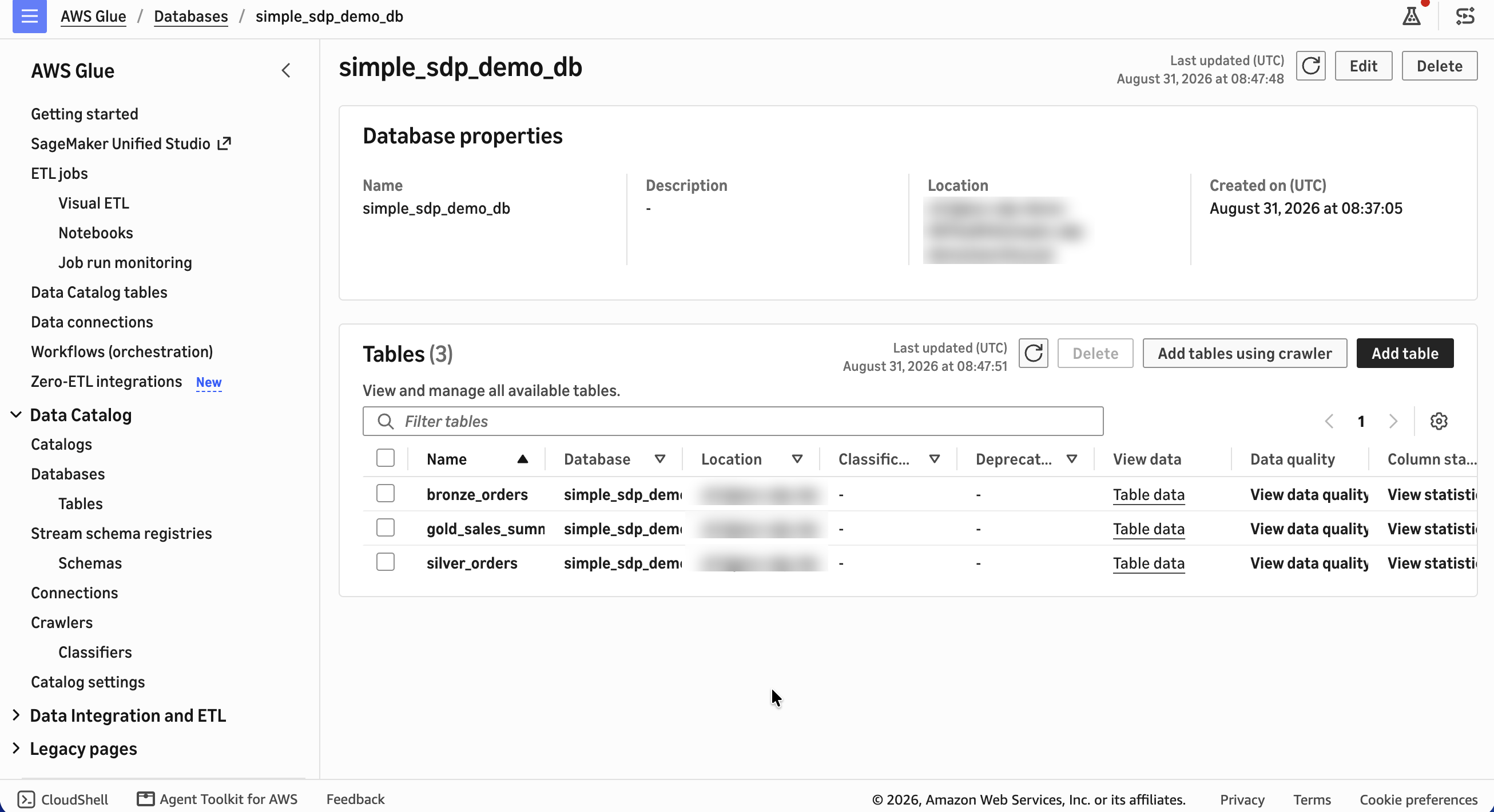
Figure 5: The three output tables in the AWS Glue Data Catalog.

Step 9 – Query results

Query the tables with Amazon Athena. If this is your first time using Athena in this Region, set an Amazon S3 query-results location for your workgroup first (Athena console, Settings). Also make sure your identity can read the simple_sdp_demo_db tables in the Data Catalog and the underlying S3 data.

-- Bronze preserves all 6 source rows
SELECT * FROM simple_sdp_demo_db.bronze_orders ORDER BY order_id;

-- Silver retains the 5 complete orders with positive amounts
SELECT * FROM simple_sdp_demo_db.silver_orders ORDER BY order_id;

-- Gold aggregates by region
SELECT * FROM simple_sdp_demo_db.gold_sales_summary ORDER BY region;

Expected gold result:

Table 3: Gold layer aggregation results by region.

Running the query in the Amazon Athena console returns the aggregated result. The following screenshot shows the gold query and its three result rows (AMER, APAC, and EMEA), matching the values in the preceding table.

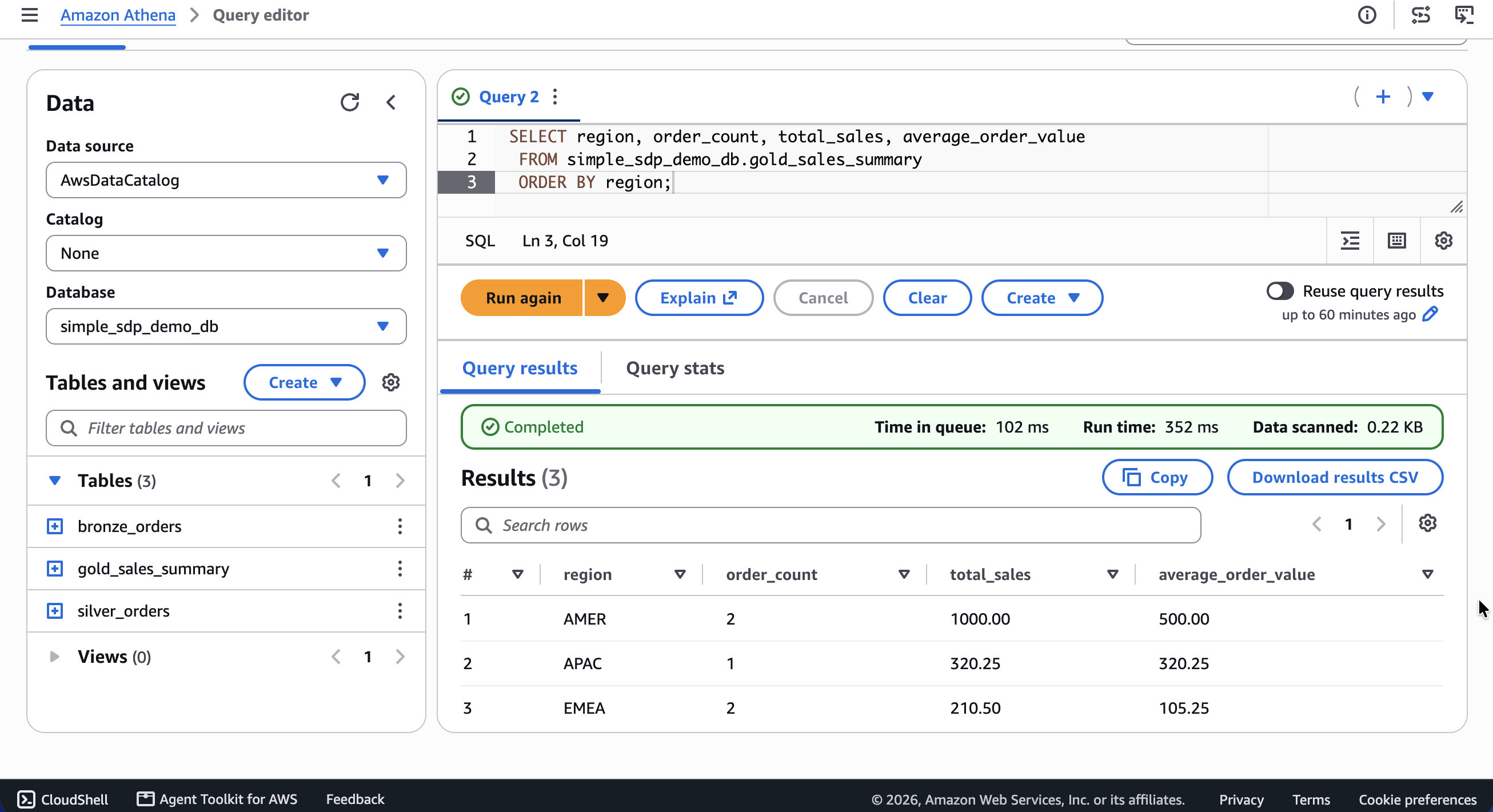
Figure 6: The gold table results in the Amazon Athena console.

Cost considerations

AWS Glue 6.0 bills ETL jobs by the data processing unit (DPU)-hour, per second, with a 1-minute minimum per run. AWS Glue 6.0 is also priced 30 percent lower per DPU-hour than AWS Glue 5.1, with no change to your workload, so the same job costs less to run on 6.0. This walkthrough runs on 2 G.1X workers (2 DPUs), reads a 6-row CSV, and completes each run in about 2 minutes. It produces three tables in one AWS Glue Data Catalog database.

To estimate the cost of a run, multiply the 2 DPUs by the run time in hours by your Region’s AWS Glue 6.0 DPU-hour rate. You can find that rate on the AWS Glue pricing page, and rates differ by AWS Region. The Amazon S3 objects created are the 6-row CSV, the pipeline zip, and the three tables’ data. To stop further charges, delete the resources when you finish, as shown in the next step.

Step 10 – Clean up

To avoid ongoing charges, delete the resources you created:

# Delete the AWS Glue job
aws glue delete-job --job-name "${JOB_NAME}" --region "${AWS_REGION}"

# Delete the Data Catalog database and its table metadata
aws glue delete-database --name "${DATABASE}" --region "${AWS_REGION}"

# Remove the S3 objects
aws s3 rm "s3://${BUCKET}/${PREFIX}/" --recursive --region "${AWS_REGION}"

What’s next

You now have a single pipeline that turns raw order records into validated, aggregated analytics tables, without writing orchestration logic. From here you can:

• Extend: Add transformation stages (additional @dp.materialized_view functions) and connect them by referencing upstream tables. The pipeline picks up the new dependency automatically.
• Scale: This walkthrough uses materialized views throughout, so every layer fully recomputes on each run (materialized views don’t support incremental refresh). To process only new data as it arrives, convert the bronze layer to a streaming table, which maintains state across runs with checkpoints. For that cross-run state to persist, a streaming table’s data and checkpoint state must not be stored locally. Hive or AWS Glue managed tables require the database’s LocationUri to point to an Amazon S3 path, while Apache Iceberg tables manage their table metadata themselves.
• Govern: Protect the Data Catalog tables SDP produces with AWS Lake Formation fine-grained access control. It enforces table-, row-, column-, and cell-level permissions on read queries in AWS Glue Spark jobs (Glue 5.0 and later, for Hive and Iceberg tables). Because this enforcement covers batch reads, it applies to SDP’s materialized views but not to streaming tables, which read through Spark Structured Streaming.
• Automate: Store the pipeline project in source control. Have your continuous integration and continuous delivery (CI/CD) pipeline package and upload it to Amazon S3 so each job run maps to a known build. Version the zip by object key, or upload the unzipped project to an S3 prefix and turn on Amazon S3 bucket versioning.
• Monitor: Use Amazon CloudWatch metrics and AWS Glue job run insights for pipeline observability, latency tracking, and failure alerting.

Conclusion

In this post, you used Spark Declarative Pipelines, the declarative alternative to explicitly orchestrated ETL, now available in AWS Glue 6.0. Two decorated Python functions and one SQL file define the bronze, silver, and gold datasets, and SDP resolves the dependencies and manages execution order for you.

With SDP, you declare what each dataset should contain and the declarative framework handles ordering and execution. A three-layer pipeline that would otherwise need separate transform and orchestration logic runs as one job that you can ship and maintain.

To get started, open the AWS Glue console and build the walkthrough pipeline, or adapt the pattern to your own bronze, silver, and gold datasets. For the full set of features, see the AWS Glue 6.0 launch announcement. To move existing jobs to the Spark 4.1 runtime, see Upgrade AWS Glue jobs to AWS Glue 6.0 with AI-powered Spark upgrades. For job configuration details, see the AWS Glue Developer Guide.

About the authors